Our capital. Your skills. Shared profits.


27K +
Active traders
200+
Trading Instruments
$1 200 000
Max. Trader Capital
Grow with us
Pass the challenge, trade with funded capital, and withdraw profits - earning rewards for your trading success


About Upscale
We bring together capital, AI, and precision execution in one prop trading platform. You get a funded trading account, the tools to grow, and transparent terms. We succeed when you succeed.


| Profit | Daily Drawdown | Total Drawdown | Profit Days | |
| Phase 1 | +5% | +5% | +10% | 3 |
| Phase 2 | +8% | +5% | +10% | 5 |
| Trading | ∞ | +5% | +10% | 5in 14 days |

$200,000
Market Legend
Participation: $1,299
$1000 for $6.495

$100,000
Top Traders' Choice
Participation: $799
$1000 for $7.99

$50,000
Confident Entry
Participation: $399
$1000 for $7.98

$25,000
Optimal
Participation: $249
$1000 for $9.96

$10,000
Smooth Start
Participation: $119
$1000 for $11.9

$5,000
Minimal Risk
Participation: $69
$1000 for $13.8

New to trading?
We’ve got you covered!
Learn everything from scratch with Storm Academy — free, flexible, and built to help you grow. Level up your skills and earn rewards as you progress!
Start learning →New to trading?
We’ve got you covered!
Learn everything from scratch with Storm Academy — free, flexible, and built to help you grow. Level up your skills and earn rewards as you progress!

Blog

Crypto Bull Run Guide: Timing, Indicators & Winning Strategies
Crypto Bull Run Guide: Timing, Indicators & Winning Strategies
Understanding crypto bull runs transforms chaos into opportunity. These periods create life-changing wealth for prepared investors. This guide reveals how to identify, navigate, and profit from the next major market surge.
⚠️ Important Disclaimer: This article analyzes historical cryptocurrency market patterns and cycles. While these patterns provide valuable frameworks for understanding market behavior, past performance never guarantees future results. Cryptocurrency markets remain highly volatile, unpredictable, and subject to regulatory changes. Each bull run cycle brings unique characteristics, external factors, and market conditions. The information presented here is educational and should not be considered financial advice. Always conduct your own research and consult with financial professionals before making investment decisions.
What is a Crypto Bull Run Meaning?
A crypto bull run represents sustained upward price momentum across digital assets. Markets rally for months. Optimism spreads like wildfire through trading communities.
The bull run meaning extends beyond simple price increases. Bitcoin often gains over 1,000% during these periods. The entire market capitalization can grow five to ten times. Volume builds gradually throughout the cycle.
True bull markets last between 12 and 18 months typically. They differ fundamentally from temporary price spikes. Market sentiment indicators like the Fear and Greed Index consistently read above 70. Capital flows steadily into crypto assets.
Key Takeaways:
- Definition: Sustained period of rising cryptocurrency prices with widespread market optimism
- Duration: Typically 12-18 months from accumulation to peak
- Bitcoin Performance: Historical gains exceeding 1,000% per cycle
- Market Growth: 5-10x increase in total market capitalization
- Sentiment: Fear and Greed Index readings consistently above 70
Market cycles follow predictable patterns. Smart money accumulates during bear markets. Retail investors enter during markup phases. Understanding these phases separates successful traders from the crowd.
Bull runs create opportunities across all market participants. Experienced traders scale positions strategically. Newcomers often chase momentum late in cycles. The difference between these approaches determines long-term success.
The Psychology Behind Bull Markets
Market psychology drives bull run dynamics more than fundamentals alone. The Fear and Greed Index measures collective emotions on a 0-100 scale. Bull markets typically show readings between 70 and 100.
During 2017's peak, the index hit extreme greed levels. Social media amplified every gain. New investors entered daily. FOMO (fear of missing out) dominated decision-making across retail traders.
The same pattern repeated in 2021. Bitcoin reached new all-time highs. Altcoins surged exponentially. Everyone became a crypto expert overnight.
These emotional shifts create both opportunity and danger. Disciplined traders recognize when euphoria reaches unsustainable levels. They protect gains while others chase tops.
Bull vs Bear Markets in Crypto
Bull and bear markets represent opposite sides of market cycles. Each phase exhibits distinct characteristics. Recognizing these differences protects capital and maximizes gains.
Bull Market Characteristics:
- Sustained uptrend lasting 12-18 months
- Gradually increasing volume with peaks at cycle tops
- Fear and Greed Index above 70 consistently
- Positive news dominates headlines
- New projects launch successfully
- Retail participation increases steadily
Bear Market Characteristics:
- Extended downtrend spanning 12-24 months
- Declining volume throughout the cycle
- Fear and Greed Index below 30
- Negative sentiment prevails
- Project failures make headlines
- Retail investors exit markets
The accumulation phase marks bear market endings. Smart money recognizes value before crowds. Prices consolidate near cycle lows. Volume remains relatively low.
Markup phases define bull markets. Public awareness grows. FOMO intensifies. Prices accelerate dramatically. This phase generates the largest gains.
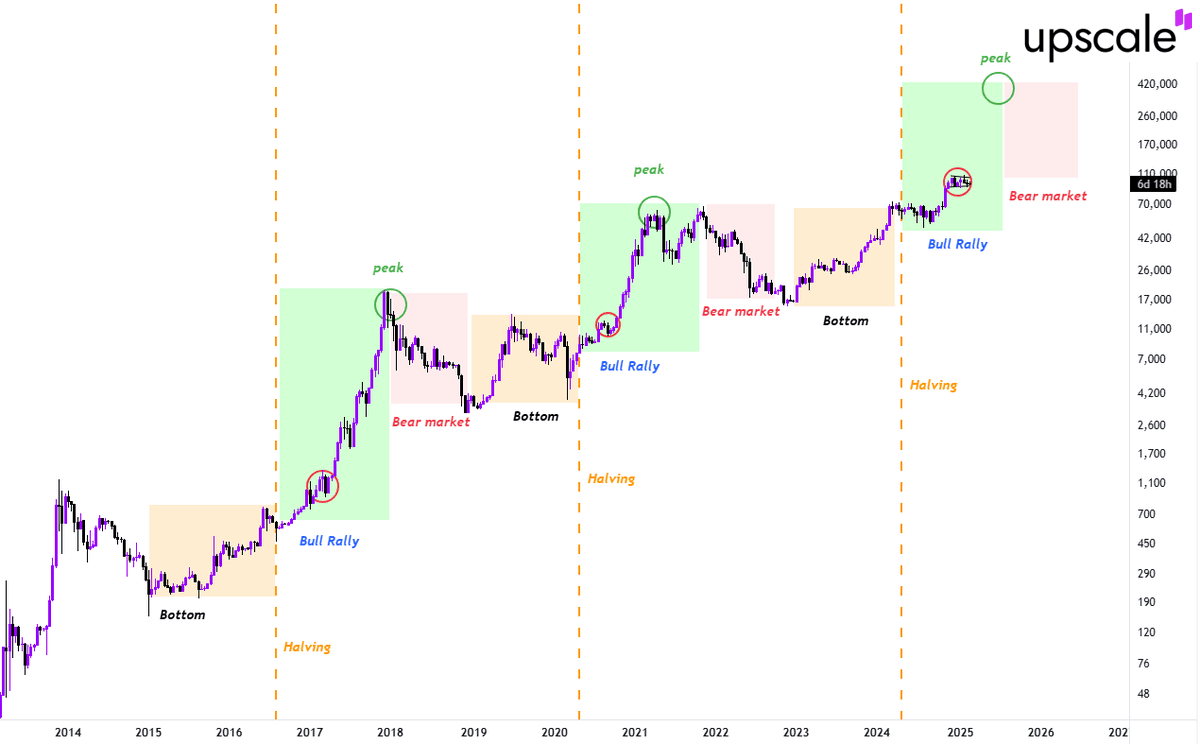
Historical Crypto Bull Run History
Cryptocurrency markets have experienced three major bull runs since Bitcoin's creation. Each cycle followed similar patterns. Each exceeded previous peaks dramatically. Studying crypto bull run history reveals consistent patterns.
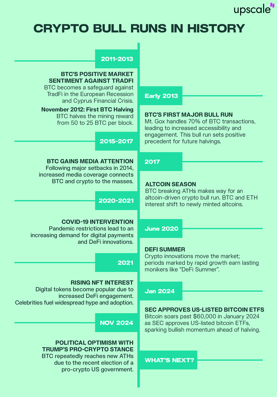 The 2013 bull run saw Bitcoin surge from $13 to $1,100. The Cyprus banking crisis drove adoption. Media coverage intensified. Retail interest exploded. This early crypto bull run history established foundational patterns.
2017's cycle proved even more spectacular. Bitcoin climbed from $1,000 to $20,000. ICOs (initial coin offerings) raised billions. Ethereum enabled smart contract platforms. Altcoins delivered life-changing returns.
The 2021 bull run marked institutional arrival. Bitcoin reached $69,000. Ethereum hit $4,800. The total crypto market cap exceeded $3 trillion. DeFi and NFTs captured mainstream attention.
Bitcoin halving events preceded each major bull run. These programmed supply reductions occur every four years. They cut new Bitcoin issuance by 50%. Supply shock dynamics then drive price appreciation.
The 2012 halving preceded the 2013 bull run. The 2016 halving led into 2017's surge. The 2020 halving sparked 2021's rally. This pattern creates predictable timing frameworks.
However, correlation does not guarantee causation. While historical patterns show consistent relationships between halvings and bull runs, numerous other factors influence market outcomes. Economic conditions, regulatory developments, technological changes, and global events all play crucial roles. Future cycles may deviate from historical norms.
Each cycle attracted larger participant bases. 2013 drew tech enthusiasts. 2017 brought retail traders. 2021 welcomed institutions. The next cycle promises even broader adoption.
 Learning from past cycles improves future positioning. Early accumulation during bear markets yields maximum returns. Patient holding through volatility preserves gains. Strategic exits near cycle peaks protect capital.
The 2021 Bull Run Case Study
The 2021 bull run demonstrated crypto's maturation. Institutional adoption reached critical mass. MicroStrategy accumulated over 100,000 Bitcoin. Tesla added Bitcoin to the corporate treasury. Square (now Block) made significant purchases.
These corporate moves validated cryptocurrency as legitimate assets. Traditional finance could no longer ignore digital currencies. Bitcoin ETF applications multiplied. Regulatory frameworks began taking shape.
Ethereum's ecosystem exploded during this cycle. DeFi protocols locked billions in value. NFT marketplaces processed record volumes. Layer-2 solutions addressed scalability challenges. The entire blockchain infrastructure evolved rapidly.
The cycle peaked in November 2021. Bitcoin reached $69,000. Market sentiment hit extreme greed. Leverage ratios climbed dangerously high. Warning signs accumulated for observant traders.
When Do Bull Runs End?
Recognizing bull market endings preserves hard-earned gains. Several reliable indicators signal approaching tops. Smart money begins exiting positions. Retail enthusiasm reaches fever pitch.
The Fear and Greed Index typically peaks between 90 and 100. Extreme greed readings warn of reversals. Historical data confirms this pattern across all major cycles.
Trading volume characteristics shift noticeably. Climax volume occurs at tops. Buying exhaustion follows. Subsequent rallies show declining participation. These technical signals provide actionable warnings.
Distribution phases unfold gradually at first. Smart money sells into strength. Prices continue rising temporarily. Eventually momentum fails. Sharp corrections begin.
Market cycle phases provide strategic frameworks. Accumulation occurs at bottoms. Markup defines bull markets. Distribution marks tops. Markdown completes the cycle. Understanding current phase positioning improves decision-making dramatically.
On-chain metrics reveal institutional behavior. Large transactions increase during distribution. Exchange inflows surge. Realized profits hit extremes. These data points confirm cycle positioning.
Successful traders prepare exit strategies long before tops. They scale out systematically. They avoid timing exact peaks. They preserve capital for next cycle accumulation.
Key Indicators of an Approaching Bull Run
Identifying early bull market signals creates significant advantages. Multiple indicators confirm emerging trends. Combining signals improves accuracy substantially.
Bitcoin halving events provide primary timing catalysts. The next halving occurred in April 2024. Historical patterns suggest bull markets begin 12-18 months post-halving. This framework guides strategic positioning.
Accumulation phase characteristics signal bull run approaches. Smart money enters quietly. Prices consolidate near cycle lows. Volume remains subdued. Retail interest stays minimal.
Fear and Greed Index readings offer sentiment insights. Extended periods below 20 indicate extreme fear. These zones historically mark excellent entry points. Transitioning from fear toward neutral suggests cycles turning.
On-chain metrics validate emerging trends. Bitcoin accumulation by long-term holders increases. Exchange balances decline as coins move to cold storage. Network fundamentals strengthen progressively.
Technical Signals to Watch For
Technical analysis provides concrete, observable signals. Chart patterns reveal market psychology. Price action reflects all available information.
Golden crosses mark powerful bullish signals. This occurs when the 50-day moving average crosses above the 200-day. Historical data confirms reliability across crypto markets.
Higher lows on weekly and monthly charts demonstrate strengthening momentum. Each correction finds support at elevated levels. This pattern validates underlying demand.
Volume analysis confirms price movements. Genuine bull runs show gradually increasing volume. Explosive volume spikes mark acceleration phases. Declining volume during rallies signals false moves.
The Connection Between Bitcoin Bull Run and Altcoin Performance
Bitcoin dominates cryptocurrency markets fundamentally. Its price movements influence all digital assets. Understanding this relationship optimizes portfolio allocation. Every bitcoin bull run creates predictable patterns.
Bitcoin typically leads bull market rallies initially. Capital flows into the most established cryptocurrency first. Risk-averse investors seek relative safety. Bitcoin's liquidity and recognition attract initial attention. The bitcoin bull run momentum then spreads to altcoins.
As Bitcoin rallies extend, profits rotate into altcoins. Traders seek higher percentage gains. Ethereum often benefits next as the second-largest cryptocurrency. Then capital spreads across smaller market cap projects.
This rotation pattern creates altcoin season. Smaller cryptocurrencies outperform Bitcoin dramatically. 3-5x multipliers above Bitcoin's gains become common. High-risk, high-reward opportunities multiply.
Understanding Altcoin Season
The altcoin season represents the most explosive bull market phase. Bitcoin's initial rally attracts attention. Profits then chase higher percentage gains elsewhere.
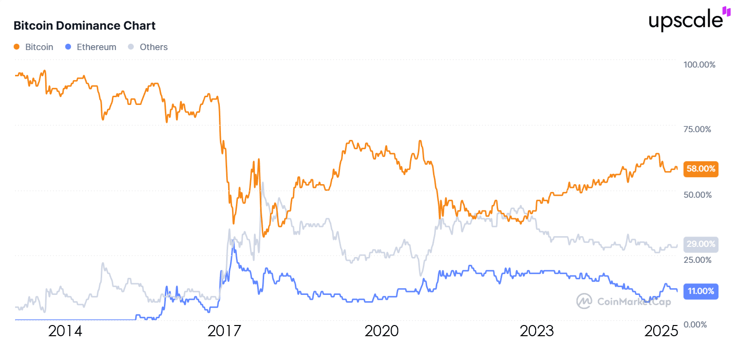
Timing altcoin season entries proves crucial. Too early means underperforming Bitcoin. Too late means buying near cycle peaks. Monitoring Bitcoin dominance charts helps identify transitions.
 Performance multipliers during altcoin seasons exceed normal market behavior. 10x, 50x, even 100x gains occur regularly. Smaller market caps allow parabolic moves. This creates both opportunity and danger.
Strategies to Capitalize During the Next Bull Run Crypto
Successful bull market navigation requires systematic approaches. Emotional decision-making destroys capital. Strategic frameworks preserve it. Understanding bull run crypto dynamics separates winners from losers.
Position building during accumulation phases provides optimal entries. Dollar-cost averaging reduces timing risk. Accumulating quality assets at cycle lows maximizes eventual returns. Patient capital captures full bull market gains when the next bull run crypto begins.
Portfolio allocation balances risk and reward. Bitcoin provides relative stability. Major altcoins like Ethereum offer enhanced upside. Selected smaller projects provide lottery tickets. Diversification across market caps spreads risk intelligently.
Entry timing uses technical and fundamental signals. Waiting for confirmation reduces false starts. Multiple indicator confluence increases probability. Strategic patience beats impulsive trading consistently.
Position sizing adapts to risk profiles. Conservative allocations favor Bitcoin and major altcoins. Aggressive approaches include more speculative positions. No single strategy suits all investors. Personal risk tolerance determines optimal allocation.
At , we understand that timing and execution are everything during crypto bull runs. As a leading crypto prop trading platform, we bring together capital, AI-powered analytics, and precision execution tools in one comprehensive solution. When you trade with a funded account from UpscaleTrade, you get the capital to maximize bull market opportunities, advanced tools to identify optimal entry and exit points, and transparent terms that align our success with yours. Our platform helps you implement the systematic strategies discussed here while managing risk effectively throughout the cycle.
Strategy Approaches Based on Risk Tolerance
| Risk Level | Bitcoin Allocation | Major Altcoins | Small Cap Altcoins | Strategy Focus | |------------|-------------------|----------------|-------------------|----------------| | Conservative | 70% | 25% | 5% | Capital preservation with steady growth | | Moderate | 50% | 35% | 15% | Balanced growth with managed risk | | Aggressive | 30% | 40% | 30% | Maximum growth potential |
Creating a Bull Market Exit Strategy
Exit strategies separate successful traders from the rest. Greed destroys more capital than fear. Predetermined targets enable disciplined execution.
Percentage-based profit taking provides systematic approaches. Sell 20% at 2x. Sell 20% more at 3x. Continue scaling systematically. This method captures gains while maintaining exposure.
Time-based exits consider cycle positioning. Historical patterns show 12-18 month bull markets. Approaching these timeframes suggests reducing exposure. Cycle awareness trumps price targeting alone.
Market sentiment indicators guide exit timing. Fear and Greed Index above 90 warns of tops. Extreme euphoria in social media signals danger. Smart money exits when retail rushes in.
Technical analysis identifies distribution phases. Volume characteristics change noticeably. Momentum indicators diverge bearishly. Support levels begin failing. These signals confirm cycle endings.
Current Analysis: Where Are We in the Crypto Next Bull Run Cycle?
Market analysis requires combining multiple frameworks. Current positioning determines optimal strategies. Understanding the cycle phase guides decision-making.
The April 2024 Bitcoin halving marked a crucial milestone. Historical patterns suggest bull markets accelerate 12-18 months post-halving. This framework places potential peak timing in late 2025 or early 2026.
Current Fear and Greed Index readings show moderate sentiment. Neither extreme fear nor extreme greed dominates. This neutral positioning suggests accumulation or early markup phase. Historical context supports this assessment.
Institutional adoption continues progressing. Bitcoin ETFs attracted billions in assets. Major financial institutions offer crypto services. Regulatory frameworks improve globally. These developments support a longer-term bullish thesis.
Technical analysis shows constructive patterns. Bitcoin consolidated after reaching new all-time highs. Altcoins demonstrate relative strength. Volume patterns suggest accumulation continues. Market structure supports bullish outlook.
Current positioning suggests an early-to-mid bull market phase. Significant upside potential remains. Corrections will occur inevitably. Long-term trajectory points upward. Strategic patience rewards prepared investors.
Common Mistakes to Avoid in a Bull Run in Stock Market and Crypto
Bull markets create both opportunity and danger. Common mistakes repeat across all cycles. Avoiding these errors preserves capital and maximizes returns.
FOMO (Fear of Missing Out) drives poor decisions. Chasing pumps near cycle peaks destroys capital. Buying after exponential moves guarantees losses. Emotional purchases rarely work. Discipline beats impulse consistently.
Overleveraging amplifies both gains and losses. Leverage works until it doesn't. One bad move liquidates entire positions. Bull markets create false confidence. Conservative leverage protects capital long-term.
Ignoring diversification concentrates risk dangerously. Single-asset concentration creates vulnerability. One project failing wipes out gains. Spreading risk across quality assets reduces exposure. Smart diversification balances concentration and protection.
Neglecting profit-taking leads to giving back gains. Paper profits disappear quickly. Systematic selling preserves real wealth. Greed convinces holders to wait for more. Markets punish this mindset eventually.
Following social media hype creates bagholders. Promoted coins dump after influencers sell. Due diligence beats tips consistently. Research-based decisions outperform hype-driven purchases. Think independently or pay the price.
Ignoring tax implications reduces net returns. Strategic selling considers tax efficiency. Timing transactions optimizes tax treatment. Professional advice saves money long-term. Planning ahead beats scrambling later.
Trading without stop-losses invites disaster. Unexpected crashes occur regularly. Protective orders limit downside. Small losses beat catastrophic ones. Risk management separates professionals from gamblers.
Looking Ahead: Predictions for the Next Crypto Bull Run
⚠️ Disclaimer: The following represents analytical frameworks based on historical patterns, not guarantees or financial advice. Market conditions change. External factors influence outcomes unpredictably. Use this information as one data point among many in your research.
Forward-looking analysis combines historical patterns with current developments. While nobody predicts perfectly, frameworks improve probability. This crypto bull run prediction synthesizes multiple data sources.
The April 2024 Bitcoin halving established primary timing catalyst. Historical patterns suggest peak timing in late 2025 through early 2026. This framework guides strategic positioning currently. Many crypto bull run prediction models point to similar timeframes.
Institutional adoption will accelerate throughout this cycle. More ETFs will launch globally. Major banks will expand crypto services. Regulatory clarity will improve. These developments support sustainable growth.
Bitcoin should lead initially as always. $100,000 marks psychological resistance. $150,000 becomes achievable during peak euphoria. Conservative estimates suggest 2-3x from current levels. Aggressive scenarios project higher.
Ethereum's ecosystem maturation drives strong performance. Scaling solutions improve dramatically. Real-world adoption increases. DeFi and NFTs continue evolving. ETH could reach the $8,000-$12,000 range.
The altcoin season will create spectacular opportunities. DeFi platforms with genuine utility will shine. Gaming and metaverse projects could explode. Infrastructure plays provide lower-risk exposure. Due diligence remains essential.
Macro factors influence crypto more than ever. Central bank policies affect risk appetite. Inflation concerns drive alternative assets. Geopolitical tensions highlight decentralization value. Broader context matters increasingly.
Technology improvements support long-term thesis. Layer-2 solutions address scalability. Interoperability improves. User experience gets better. Real-world utility increases. Fundamentals strengthen progressively.
Cycle characteristics may differ from the past. Institutional participation provides stability. Volatility might decrease somewhat. Bull market duration could extend. Previous patterns guide but don't guarantee. Flexibility beats rigid expectations.
FAQ
What is a crypto bull run?
A crypto bull run is a sustained period of rising cryptocurrency prices accompanied by widespread market optimism. These cycles typically last 12-18 months and feature significant capital inflows, increasing trading volume, and positive sentiment indicators. Bitcoin often gains over 1,000% during bull runs, while the entire market capitalization can grow 5-10x from bottom to peak.
When will the next crypto bull run begin?
The next crypto bull run likely began following Bitcoin's April 2024 halving. Historical patterns show bull markets accelerate 12-18 months after halving events. Current market structure, institutional adoption trends, and on-chain metrics suggest we're in early-to-mid bull market phase, with potential peak timing in late 2025 or early 2026.
How long do crypto bull runs typically last?
Crypto bull runs typically last between 12 and 18 months from the initial accumulation phase to the final distribution phase. However, the most explosive gains often occur in the final 6-8 months. The 2013, 2017, and 2021 cycles all followed similar timeframes, though exact durations varied. Understanding cycle timing helps optimize entry and exit strategies.
What are the signs of a crypto bull run?
Key signs include Bitcoin halving events, Fear and Greed Index readings consistently above 70, golden crosses on major moving averages, increasing trading volume, institutional adoption announcements, and strong on-chain metrics showing accumulation. Technical patterns like higher lows, breakouts from consolidation, and bullish divergences also signal emerging bull markets.
How does the Bitcoin halving cycle affect crypto bull runs?
Bitcoin halving events occur every four years and reduce new Bitcoin issuance by 50%. This programmed supply shock creates fundamental catalysts for bull runs. Historical data shows all three major crypto bull runs (2013, 2017, 2021) occurred 12-18 months after halving events. The April 2024 halving positioned the market for the next bull cycle.
Conclusion
Crypto bull runs create extraordinary wealth-building opportunities. Understanding cycle phases, recognizing signals, and implementing systematic strategies maximize returns while managing risk. The next bull run offers similar potential to previous cycles, but only prepared investors capture full gains.

Smart Money Concept: How to Trade Like Institutional Investors in 2025
Smart Money Concept: How to Trade Like Institutional Investors in 2025
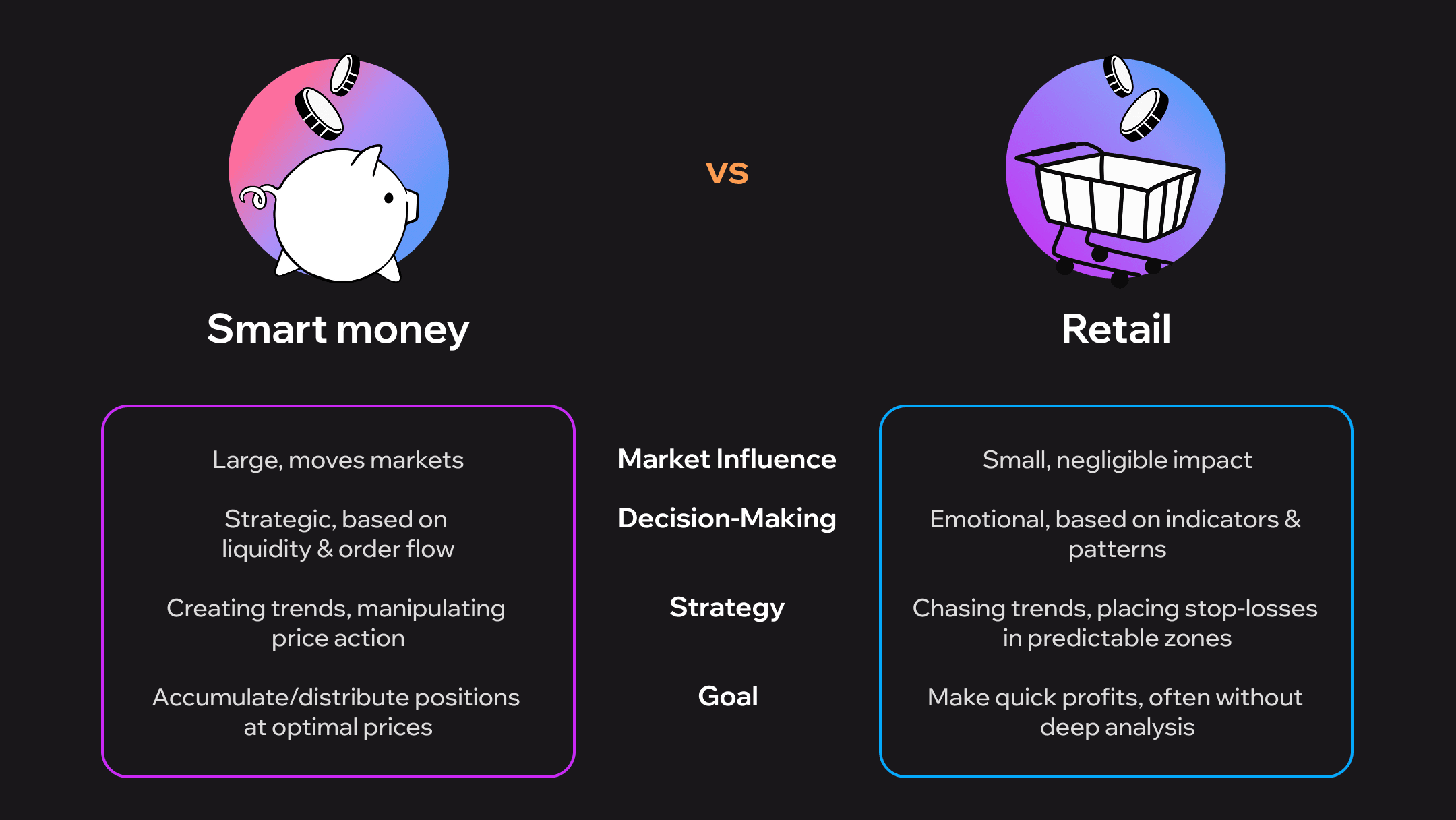
Smart Money Concept (SMC) represents a fundamental shift in how retail traders approach financial markets. Unlike traditional technical analysis that relies on lagging indicators like moving averages or RSI, SMC trading focuses on reading institutional order flow and understanding how large market participants manipulate price before executing their positions. This methodology teaches traders to identify the footprints that banks, hedge funds, and institutional investors leave in the market through order blocks, liquidity grabs, and fair value gaps.
The core principle behind smart money concept trading centers on a simple reality: institutional investors move markets, while retail traders react to those movements. By learning to recognize where institutions are likely to enter and exit positions, traders gain a significant edge over those using conventional technical analysis. The learning curve for mastering SMC typically spans six to twelve months of dedicated practice, but the methodology proves effective across multiple timeframes from M15 charts up to daily analysis. Success rates with proper risk management consistently fall within the 60-75% range, making SMC one of the most reliable trading frameworks when applied systematically.
Modern trading platforms have made implementing smart money concept strategies more accessible than ever. Traders can now analyze institutional behavior patterns, identify key liquidity zones, and execute precision entries based on order flow analysis. The methodology works equally well across forex pairs, cryptocurrency markets, and traditional stock indices, though each market presents unique characteristics in how institutions operate.
Core Smart Money Concept Components
Understanding the fundamental building blocks of smart money concept creates the foundation for successful institutional-style trading. These components work together to reveal where large market participants have placed their orders and how they intend to move price.
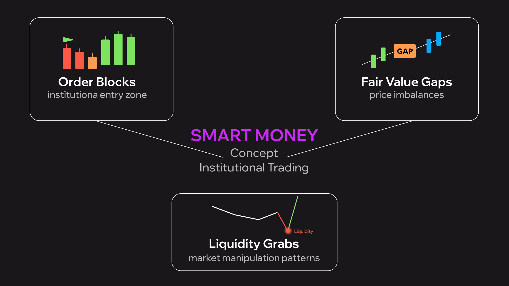
Order Blocks - Institutional Entry Zones
Order blocks represent the last opposing candle before a significant price move and identify areas where institutional orders were placed. When banks and hedge funds enter large positions, they cannot simply execute market orders without causing massive slippage. Instead, they accumulate positions over time, creating distinctive price patterns that SMC traders learn to recognize.
Bullish order blocks form when a down candle is followed by a strong upward move, indicating institutions finished selling and began aggressive buying. Bearish order blocks appear when an up candle precedes a sharp decline, showing where institutions completed their buying before initiating short positions. The key to identifying valid order blocks lies in the impulsive move away from the zone. Institutional orders create explosive price action because of the sheer volume being executed.
Smart money concept order blocks function differently from traditional support and resistance. Rather than zones where price repeatedly bounces, order blocks represent unfilled institutional orders waiting to be matched. When price returns to these zones, institutions add to their positions, creating strong reactions. Traders using platforms with advanced charting capabilities can mark these zones precisely and set alerts for when price approaches, allowing for systematic entry strategies based on institutional behavior rather than lagging technical indicators.
Fair Value Gaps and Market Structure
Fair value gaps emerge when price moves so rapidly that it leaves inefficiencies in the market structure. These gaps appear as spaces on the chart where no trading occurred at certain price levels, creating imbalances that the market typically seeks to fill. In smart money concept methodology, fair value gaps represent areas where institutional orders overwhelmed available liquidity, causing price to jump without normal auction process.
Market structure analysis within SMC focuses on identifying higher highs, higher lows, lower highs, and lower lows to determine trend direction and strength. Break of structure (BOS) occurs when price definitively breaks through a previous high or low, confirming trend continuation. Change of character (ChoCH) happens when price breaks counter to the established trend, signaling potential reversals. These structural breaks often coincide with fair value gaps, as institutions execute large enough orders to both break structure and create price inefficiencies simultaneously.
Understanding how fair value gaps interact with market structure provides traders with high-probability zones for entries. When price pulls back to fill a gap within a bullish market structure, it creates optimal long entry opportunities. Conversely, rallies into bearish fair value gaps during downtrends offer ideal short positions. The combination of structural analysis and gap identification separates smart money concept from basic price action trading.
Liquidity Grabs - Reading Institutional Manipulation
Liquidity grabs represent one of the most powerful concepts in smart money trading methodology. Institutions need substantial liquidity to fill their large orders, and that liquidity sits just beyond obvious support and resistance levels where retail traders place their stop losses. Before making major moves, smart money will often push price beyond these levels to trigger retail stops, creating the liquidity pool they need for their actual positions.
Classic liquidity grab patterns include stop hunts below recent lows in uptrends and raids above recent highs in downtrends. These moves appear designed to shake out retail traders before price reverses sharply in the intended direction. Confirmation signals include rapid reversals on high volume, engulfing candles that reclaim the broken level, and immediate movement back into the prior range. Traders who recognize these patterns avoid getting stopped out and can even enter positions in the direction of the true institutional move.
Smart Money Concept Trading Strategy Framework
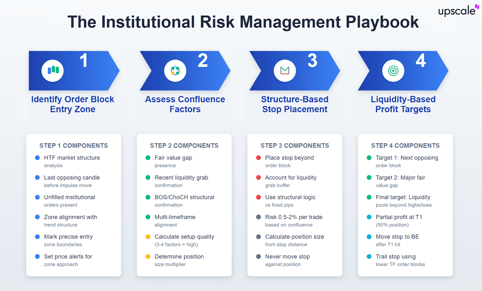
Implementing smart money concept trading requires a systematic framework that combines all core components into a coherent strategy. The process begins with multi-timeframe analysis, typically starting on daily or four-hour charts to identify overall market structure and trend direction. Traders mark key order blocks, fair value gaps, and liquidity zones on higher timeframes before drilling down to lower timeframes for precise entries.
Entry rules within the SMC trading framework demand confluence between multiple factors. An ideal entry occurs when price reaches a higher timeframe order block within market structure, creating a fair value gap on the entry timeframe, after sweeping liquidity from obvious levels. This confluence significantly increases probability compared to single-factor entries. Traders wait for confirmation through candlestick patterns, typically seeking engulfing candles or strong closes back into the order block zone before executing positions.
Exit criteria focus on logical profit targets rather than arbitrary risk-reward ratios. The first target typically sits at the next opposing order block or fair value gap, while final targets aim for major liquidity pools beyond obvious highs or lows. Stop losses are placed beyond the order block being traded, accounting for potential liquidity grabs that might occur before the main move. This approach aligns exits with where institutions are likely to take profits rather than using round numbers or fixed percentages that lack market structure context.
Position sizing in smart money concept trading follows institutional risk management principles. Rather than risking fixed percentages on every trade, SMC practitioners scale position sizes based on confluence factors and setup quality. High-confluence setups with multiple confirming factors warrant larger positions, while lower-probability trades receive reduced capital allocation. This variable position sizing approach mirrors how institutional traders allocate capital across opportunities with varying conviction levels.
SMC vs Traditional Trading Methods
 The distinction between smart money concept and traditional technical analysis extends far beyond simple terminology differences. Traditional trading relies heavily on lagging indicators that calculate values from past price data. Moving averages, MACD, RSI, and similar tools all react to price movements that already occurred, creating inherent delays in signal generation. By the time these indicators trigger entries, institutions have often already positioned themselves and begun taking profits.
Smart money concept trading operates proactively rather than reactively. By identifying where institutions must go to find liquidity and fill orders, SMC traders position themselves ahead of major moves rather than chasing momentum after it develops. This fundamental difference in approach explains why SMC practitioners often enter positions that appear counterintuitive to traditional technical traders. When conventional analysis shows oversold conditions suggesting bounces, SMC traders recognize liquidity grabs preparing for further declines.
Supply and demand trading represents the closest traditional methodology to smart money concept, as both focus on identifying zones where significant orders exist. However, supply and demand typically treats these zones as static areas where price repeatedly reacts, while SMC recognizes the dynamic nature of institutional order flow. Order blocks represent unfilled orders that institutions actively manage, adjusting positions as market conditions evolve. This nuanced understanding allows SMC traders to distinguish between zones that will hold and those likely to break as institutional sentiment shifts.
The effectiveness gap between methodologies becomes evident in ranging markets where traditional technical analysis struggles. Indicators generate conflicting signals in consolidation, while smart money concept clearly identifies the liquidity zones institutions are targeting and the order blocks they're building positions from. This advantage proves particularly valuable for traders seeking consistency across varying market conditions.
Market-Specific Applications
Smart Money Concept in Forex Trading
Foreign exchange markets provide ideal conditions for smart money concept application due to the massive institutional participation required for currency transactions. Central banks, commercial banks, and multinational corporations constantly execute large currency orders, creating clear order blocks and liquidity patterns. Major pairs like EURUSD, GBPUSD, and USDJPY display particularly clean SMC setups because of the concentrated institutional flow and high liquidity that prevents excessive manipulation.
The forex market's 24-hour nature allows traders to identify institutional order flow across different trading sessions. London and New York sessions typically show the most significant smart money activity, with clear liquidity grabs occurring during session opens as institutions position for the day ahead. Currency pairs often respect order blocks for extended periods because institutional forex positions remain active for days or weeks, creating reliable zones for multiple entry opportunities. Traders implementing smart money concept forex strategies focus on higher timeframe structure while using M15 or M30 charts for entries, aligning with the methodical pace at which institutions build currency positions.
Day Trading with Smart Money Concept
Applying smart money concept to day trading requires adjustments in timeframe focus while maintaining the same core principles of reading institutional behavior. Day traders typically work with M5 to M15 charts for entries while referencing H1 and H4 for structure and order block identification. The faster timeframes demand quicker decision-making, but the advantage comes from catching institutional moves within a single session rather than holding positions overnight.
Intraday smart money concept patterns often revolve around liquidity grabs at the beginning of major sessions. The Asian session low frequently gets swept during London open as institutions collect stops before pushing price higher, creating classic SMC entry setups. Similarly, New York open commonly sees raids of European session highs or lows before the true directional move emerges. Day traders who understand these patterns position themselves to capitalize on the reversals that follow liquidity collection.
The compressed timeframes in day trading amplify the importance of execution precision. Entries must occur at the exact edge of order blocks rather than anywhere within the zone, and stops need tight placement to maintain favorable risk-reward on shorter-term moves. Modern trading platforms with one-click execution and precise order placement capabilities become essential tools for implementing SMC day trading strategies effectively. Traders can practice these faster-paced setups through demo accounts before committing capital to live markets where execution speed directly impacts profitability.
Risk Management for SMC Trading
 Institutional-style risk management separates consistently profitable smart money concept traders from those who struggle despite understanding the technical concepts. Unlike retail risk management that focuses primarily on percentage-based stop losses, SMC risk management considers market structure context and institutional behavior patterns when determining position parameters.
Stop loss placement in smart money trading always accounts for potential liquidity grabs beyond the order block being traded. Rather than placing stops at obvious levels like just below order block lows, institutional-minded traders add buffer room for wicks that might sweep stops before reversing. This approach accepts slightly wider stops in exchange for avoiding premature exits on positions that ultimately work. The trade-off makes sense because SMC entries occur at structural levels where directional conviction runs high, justifying the additional risk to avoid manipulation-induced stop outs.
Position sizing methodology within smart money concept adjusts based on setup confluence and conviction level. When multiple factors align including higher timeframe order blocks, fair value gaps, market structure confirmation, and liquidity grab evidence, traders can comfortably increase position sizes because probability dramatically improves with confluence. Conversely, trades based on single factors receive minimum position sizing. This variable approach ensures capital allocation matches opportunity quality rather than treating every setup identically.
The risk-reward framework in SMC trading differs fundamentally from traditional fixed-ratio approaches. Rather than targeting arbitrary 2:1 or 3:1 ratios, institutional-style traders identify logical profit targets based on market structure. The first target typically sits at the next opposing order block or major fair value gap, while final targets aim for liquidity pools beyond obvious structural levels. This structure-based targeting often yields reward-to-risk ratios exceeding 5:1 or even 10:1 on well-executed trades, though the focus remains on structural logic rather than ratio achievement.
Advanced SMC Psychology and Implementation
Mastering the smart money concept extends beyond technical pattern recognition into understanding the psychological dynamics between institutional and retail participants. Institutions deliberately engineer price action to trigger emotional responses in retail traders, creating the liquidity and positioning they need for their actual trades. Recognizing this manipulation while avoiding emotional reactions separates successful SMC implementation from theoretical knowledge.
Breaker blocks represent an advanced SMC concept where previously bullish order blocks fail and become bearish zones, or vice versa. This occurs when institutional sentiment shifts significantly enough that former support becomes resistance. Traders who adapt to these breaker patterns avoid fighting against repositioned institutional flow. The psychology behind breaker blocks centers on recognizing when market narrative changes demand strategic flexibility rather than stubbornly holding bias.
Mitigation blocks function similarly to order blocks but represent areas where institutions need to mitigate existing positions before establishing new directional trades. These zones often appear as minor pullbacks within strong trends where smart money takes partial profits or adjusts positions before the next leg. Understanding mitigation versus primary order blocks prevents confusion about which zones will hold for major reversals versus brief pauses in existing trends.
Implementation framework for systematic smart money concept practice begins with paper trading or demo account work until pattern recognition becomes second nature. Traders should mark order blocks, fair value gaps, and liquidity zones in real-time daily, then review how price interacted with those levels after the fact. This deliberate practice builds the pattern recognition neural pathways required for live trading success. Progressing to live markets should start with minimum position sizes, gradually scaling up as consistency develops over months rather than rushing into full-size positions immediately.
Conclusion - Your SMC Action Plan
Smart money concept provides retail traders with a framework for understanding and trading alongside institutional participants rather than being their counterparty. The methodology's effectiveness stems from its foundation in market mechanics and order flow reality rather than mathematical indicators divorced from actual buying and selling pressure.
Your path forward starts with education and practice. Begin by studying price charts through the SMC lens, identifying order blocks, fair value gaps, and liquidity grabs on instruments you plan to trade. Mark these levels in advance and observe how price reacts when reaching them. This observational practice builds intuition faster than theoretical study alone. Consider structured learning through quality educational resources or mentorship programs that provide feedback on your analysis, accelerating the pattern recognition development process.
Implementation should progress methodically from paper trading through small live positions to full-size trading only after demonstrating consistent profitability. The journey from learning smart money concept to mastering its application typically requires six to twelve months of dedicated effort, but the resulting edge in understanding market mechanics provides lasting competitive advantages. Trading platforms with advanced charting, precise execution capabilities, and comprehensive order management tools support this implementation journey by allowing you to focus on analysis and decision-making rather than fighting technology limitations.
Trading like institutional investors in 2025 means mastering Smart Money Concepts — understanding order blocks, liquidity zones, and institutional footprints on the chart. With , traders can apply these methodologies using AI-powered analytics and real-time order flow data, scaling their strategies with company capital and transparent profit-sharing. This integration allows retail traders to align with institutional moves, execute with precision, and maximize returns in volatile markets.
FAQ
How do I identify valid order blocks in smart money concept trading?
Valid order blocks show specific characteristics including an impulsive move away from the zone, clean candle structure without excessive wicks, and positioning within broader market structure context. The candle preceding the impulse should have clear rejection from one direction followed by explosive movement opposite. Higher timeframe order blocks carry more significance than lower timeframe ones, and blocks forming after liquidity grabs prove more reliable than random swing points. Confluence with fair value gaps or major structural levels strengthens order block validity considerably.
What's the typical success rate with SMC trading strategies?
Smart money concept trading achieves win rates between 60-75% when implemented with proper risk management and selective trade filtering. Success rates improve significantly when traders demand confluence between multiple factors rather than taking every potential setup. The methodology's strength lies not just in win rate but in favorable risk-reward profiles, as structure-based targeting often yields ratios exceeding 3:1 or 5:1. Consistency develops over time as pattern recognition improves through deliberate practice and market observation.
Can I use smart money concept with small trading accounts?
SMC works effectively with accounts of any size because the methodology focuses on percentage-based risk management rather than absolute position sizes. Small accounts benefit particularly from SMC's high-probability setups and favorable risk-reward profiles, allowing capital growth through consistent execution. The key lies in accepting position sizes appropriate to account balance rather than over-leveraging to achieve arbitrary profit targets. Starting with micro lots or cent accounts while learning prevents significant capital loss during the skill development phase.
How does smart money concept differ from supply and demand trading?
While both methodologies identify zones where significant orders exist, smart money concept recognizes the dynamic nature of institutional order flow versus static supply-demand zones. SMC incorporates liquidity grabs, fair value gaps, and changing market structure into analysis, while traditional supply-demand focuses primarily on reaction zones. Smart money traders understand that institutions actively manage positions and create manipulation patterns before major moves, adding layers of analysis beyond basic zone identification.
What technical indicators complement smart money concept analysis?
Smart money concept functions as a complete standalone methodology requiring no indicators, as it focuses on pure price action and order flow. Some traders incorporate volume analysis or VWAP to confirm institutional participation levels, but lagging indicators like moving averages or oscillators typically conflict with SMC principles. The methodology's strength lies in reading price structure directly rather than filtering it through mathematical transformations that introduce lag and reduce clarity.
Is smart money concept suitable for complete trading beginners?
SMC presents a steeper initial learning curve than basic technical analysis because it requires understanding market mechanics and institutional behavior rather than simply following indicator signals. However, beginners who commit to proper education often develop better trading foundations through SMC than those starting with indicator-dependent approaches. The six to twelve month mastery timeline assumes consistent study and practice, making structured learning programs valuable for accelerating the education process and avoiding common misconceptions that delay progress.
Where can I find quality smart money concept learning resources?
Quality SMC education comes from sources emphasizing practical application over theoretical discussion. Look for programs providing chart examples, trade breakdowns, and feedback on student analysis rather than vague conceptual explanations. Many successful SMC traders share educational content through various platforms, though distinguishing between quality instruction and superficial coverage requires careful evaluation. Consider starting with free resources to grasp core concepts before investing in comprehensive courses or mentorship that provide structured learning paths and personalized guidance for skill development.

Best Scalping Trading Strategies for Quick Profits
Best Scalping Trading Strategies for Quick Profits
You already know what scalping is. Now you need proven strategies that actually work. This guide delivers eight complete methods with exact parameters — entry rules, exit criteria, indicator settings, and performance metrics. No theory. Just actionable approaches ready to implement. Professional scalpers maintain a strategy arsenal. They deploy specific methods matching current market conditions. That's what separates winners from strugglers. Let's explore the strategies that produce quick profits when executed correctly.
Strategy Selection Framework: Matching Methods to Market Conditions
No single strategy works universally. Markets shift between trending, ranging, volatile, and calm. Successful scalpers assess market character using quantifiable metrics before entering positions.
Framework Structure:
- High Volatility + Strong Trend → Momentum breakout strategies
- High Volatility + No Clear Trend → Volatility breakout strategies
- Low Volatility + Established Range → Mean reversion strategies
- Moderate Volatility + Weak Trend → Hybrid approaches
Quantifiable Thresholds:
Strong Trend = ADX above 25. High Volatility = Current ATR exceeds 130% of 20-period average. Range-Bound = Bollinger Band width below 50% of 3-month average.
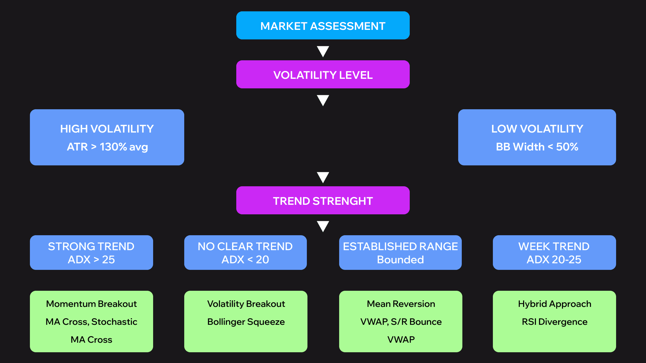 Forcing momentum strategies onto ranging markets destroys accounts. Trying mean reversion during strong trends creates losses. Match your method to conditions. Start each session with a 5-minute market assessment. Check ADX for trend strength. Measure ATR for volatility. Observe Bollinger Band width. Then select your strategy arsenal for the day.
The Best Scalping Strategies: Complete Implementation Guide
Eight complete strategies follow. Each provides exact specifications. You'll get timeframes, indicator settings, entry rules, exit criteria, optimal instruments, and expected performance.
Strategy #1 - Moving Average Crossover Strategy
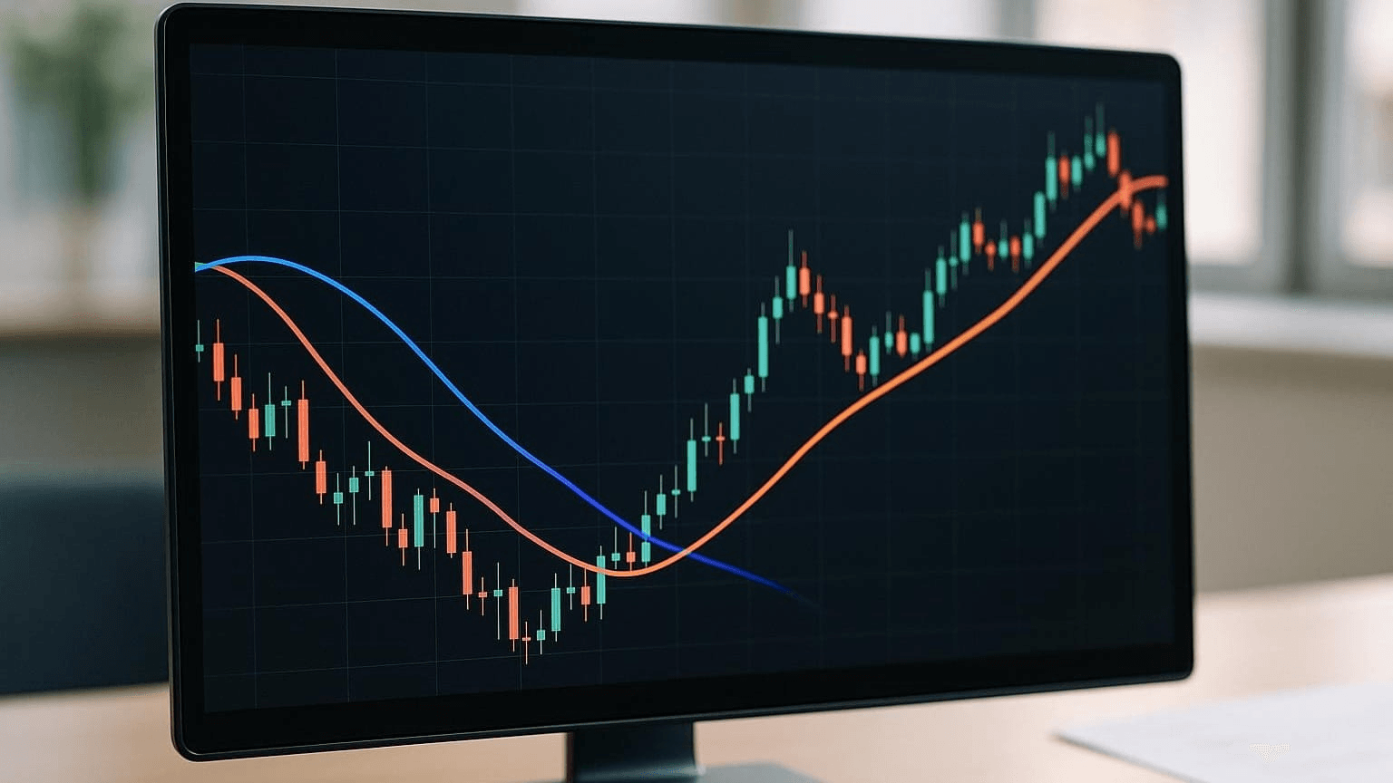 Timeframes: 5-minute analysis, 1-minute execution
Indicators: 8 EMA, 21 EMA, Volume (20-period average), RSI(7)
Entry (LONG): 8 EMA crosses above 21 EMA on 5-min. Both EMAs are sloping upward. RSI(7) above 50. Volume exceeds 120% average. Price pulls back to 8 EMA on 1-min. Enter on bounce with a bullish candle.
Exit: Target 1.5x ATR(14). Exit if 8 EMA crosses back below 21 EMA. Time-based exit after 20 minutes.
Stop Loss: 0.5x ATR(14), typically 5-8 pips EUR/USD
Risk-Reward: 1:1.5 minimum, targeting 1:2
Optimal Instruments: EUR/USD, GBP/USD, USD/JPY (London/NY overlap). BTC/USDT, ETH/USDT. SPY, QQQ, high-volume tech stocks.
Performance: 58-63% win rate. 1.7-2.1 profit factor. 8-15 minutes average duration. 8-15 trades per session.
Best Conditions: Clear trending markets with momentum during major session overlaps.
Strategy #2 - Bollinger Band Squeeze Strategy
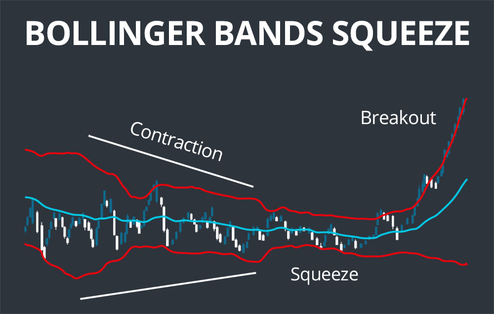 Timeframes: 3-minute primary
Indicators: Bollinger Bands (20,2), BB Width indicator, MACD (12,26,9), Volume (20-period average)
Entry (LONG): BB Width reaches 3-month low. Bands begin expanding. Price closes outside upper BB. MACD histogram turns positive and increasing. Breakout candle volume exceeds 150% average. Enter the next candle at market or limit at previous high.
Exit: Target opposite BB (full band width move). Alternative 2x ATR if the band is too wide. Move stop to breakeven after 1x ATR profit. Time limit 25 minutes.
Stop Loss: Inside squeeze range, typically 0.7x ATR
Risk-Reward: 1:2 to 1:3 (band width dependent)
Optimal Instruments: Major forex pairs during pre-news periods. ETH/USDT, BNB/USDT during consolidation. AAPL, MSFT, TSLA intraday consolidations.
Performance: 55-60% win rate. 2.0-2.5 profit factor. 12-20 minutes duration. 3-6 quality setups per session.
Best Conditions: Low volatility consolidation periods before expansion.
Strategy #3 - RSI Divergence Trading Strategy
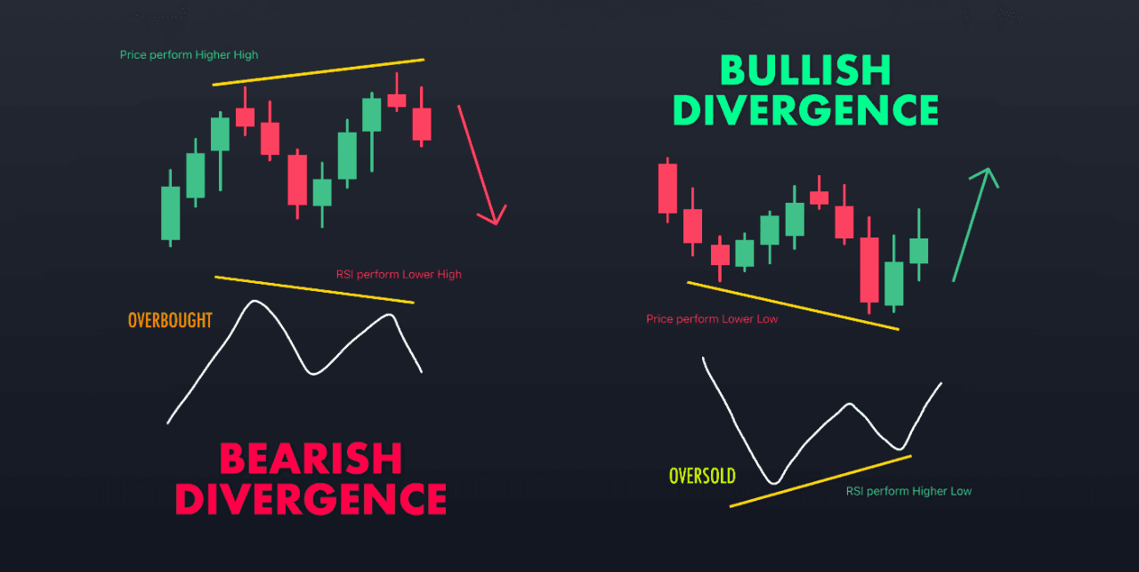 Timeframes: 5-minute for divergence identification, 1-minute for entry timing
Indicators: RSI(7), Price action (swing highs/lows), 50 EMA, Stochastic(5,3,3)
Entry (LONG - Bullish Divergence): Price below 50 EMA making lower lows. RSI simultaneously making higher lows (divergence). Price reaches support or RSI below 30. Wait for RSI to cross above 30. Stochastic crosses up from oversold on 1-min. Enter with bullish candle confirmation.
Exit: Primary target 50 EMA. Alternative 1.5x ATR if EMA distant. Close 50% at 1x ATR, hold 50% to target. Exit if divergence invalidates.
Stop Loss: Beyond swing extreme (support level)
Risk-Reward: 1:2 minimum, often 1:3+
Optimal Instruments: GBP/JPY, EUR/JPY. Altcoins during corrections. Individual stocks during intraday pullbacks.
Performance: 65-70% win rate. 2.3-2.8 profit factor. 15-30 minutes duration. 2-4 high-quality setups per session.
Best Conditions: Corrective phases within larger trends, overextended markets.
Mastering Complex Strategies with Professional Infrastructure
Complex multi-indicator strategies demand a proper trading environment. Most scalpers face barriers: insufficient capital for position sizing, lack of institutional-grade execution, challenges managing real-time risk across strategies. eliminates these obstacles with institutional infrastructure designed for high-frequency trading. Access the capital and technology to implement sophisticated scalping approaches effectively across crypto and traditional markets. Professional tools enable strategy execution with optimal quality and comprehensive analytics for continuous refinement. Focus on trading — not infrastructure concerns.
Strategy #4 - VWAP Mean Reversion Strategy
 Timeframes: 2-minute chart
Indicators: VWAP (standard), VWAP deviation bands (1σ, 2σ), Volume, 20 EMA
Entry (LONG): Price deviates 2+ standard deviations below VWAP. Volume spike confirms overextension (200%+ average). Price shows rejection wicks (buying pressure). Enter when price closes back inside the 2σ band heading toward VWAP. 20 EMA supports direction.
Exit: Primary VWAP line. Extended to the opposite 1σ if momentum strong. Move to breakeven at +50% profit. Time-based exit after 20 minutes.
Stop Loss: Beyond 2.5σ band (setup invalidation)
Risk-Reward: 1:2 to 1:4 (deviation dependent)
Optimal Instruments: High-volume stocks (AAPL, MSFT, AMZN). BTC/USDT during regular hours. ES, NQ futures during liquid sessions.
Performance: 62-68% win rate. 2.4-3.0 profit factor. 10-18 minutes duration. 4-8 opportunities per session.
Best Conditions: Normal distribution days, avoid major news events.
Strategy #5 - Support and Resistance Bounce Strategy
 Timeframes: 15-minute for level identification, 1-minute for entry precision
Indicators: Horizontal S/R levels, Price action patterns, Volume, Optional 200 SMA
Entry (LONG at Support): Identify tested support from 15-min (minimum 3 prior touches). Price approaches on decreasing momentum. Wait for rejection pattern on 1-min: hammer, bullish engulfing, pin bar (lower wick 2x+ body length). Volume on rejection exceeds 130% average. Enter at rejection candle close or next open.
Exit: Target mid-range or next technical level. Alternative 2x ATR. Trail to breakeven after 1x ATR profit. Exit if price closes beyond level.
Stop Loss: 3-5 pips beyond S/R level (tight)
Risk-Reward: 1:2 to 1:3
Optimal Instruments: EUR/USD, USD/JPY during Asian/London. BTC/USDT, ETH/USDT at established levels. High-liquidity stocks with clear ranges.
Performance: 60-65% win rate. 2.0-2.6 profit factor. 10-20 minutes duration. 3-7 level tests per session.
Best Conditions: Range-bound markets, avoid strong breakouts.
Strategy #6 - Stochastic Momentum Strategy
 Timeframes: 3-minute primary
Indicators: Stochastic (5,3,3), 21 EMA, ADX(14), Volume
Entry (LONG): Price above 21 EMA (trend filter). ADX above 20 (strength filter). Stochastic drops into oversold (below 20). K crosses above D while oversold. Volume on cross exceeds average. Enter at market on cross completion.
Exit: Primary opposite stochastic cross (K crosses back below D). Alternative stochastic reaches opposite extreme (80+ for longs). Profit target 1.5x ATR if no cross. Time limit 15 minutes.
Stop Loss: Recent swing low/high on 3-min, typically 0.6x ATR
Risk-Reward: 1:1.5 to 1:2
Optimal Instruments: All major forex pairs during trends. Major crypto pairs during directional moves. Momentum stocks during trend hours (10 AM-2 PM).
Performance: 57-62% win rate. 1.8-2.3 profit factor. 8-12 minutes duration. 10-18 opportunities per session (high frequency).
Best Conditions: Trending intraday environments with periodic pullbacks.
Strategy #7 - News Spike Fade Strategy
 Timeframes: 1-minute for rapid execution
Indicators: Economic calendar, ATR(14), Bollinger Bands (20,2), Volume, RSI
Entry (FADE - Contrarian): Identify high-impact news (NFP, CPI, Fed decisions). Allow initial spike (first 1-3 minutes post-release). Wait for the first pullback candle. Spike magnitude must exceed 2x average ATR. Enter counter-trend when: price shows rejection candle, volume declining from peak, RSI shows divergence from extreme.
Exit: Target 50% retracement of spike (Fibonacci 50%). Alternative pre-news level. Aggressive 61.8% retracement if momentum is strong. Emergency exit if new extreme beyond spike.
Stop Loss: Beyond spike extreme plus 5 pips
Risk-Reward: 1:2 to 1:4 (spike dependent)
Optimal Instruments: Forex pairs directly affected (USD pairs for US data). BTC/USDT during major announcements. Avoid stocks (gaps).
Performance: 52-58% win rate. 2.5-3.5 profit factor. 20-45 minutes duration. 1-3 major events daily.
Best Conditions: High-impact scheduled news with clear overreactions.
Strategy #8 - Opening Range Breakout (ORB) Strategy
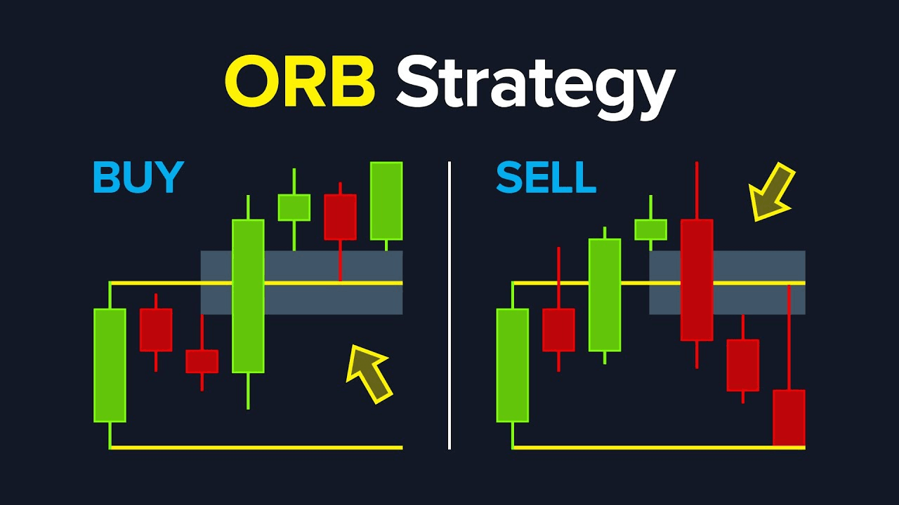 Timeframes: 30-minute for range establishment, 2-minute for entry execution
Indicators: First 30-min high/low (09:30-10:00 EST stocks, 08:00 GMT forex), ATR(14), Volume profile
Entry (LONG - Upside Breakout): Mark first 30-minute high/low. After 10:00 AM, wait for the price to approach range high. Breakout requirements: strong close above (not just wick), volume exceeds 150% opening range average, no immediate rejection (next candle continues). Enter at breakout close or next open.
Exit: Target 100% of opening range height projected from breakout. Alternative 2x range height if momentum is exceptional. Move to breakeven after 50% target achieved. Close before lunch (12:00 PM).
Stop Loss: Inside range, typically at midpoint
Risk-Reward: 1:2 typical (range dependent)
Optimal Instruments: SPY, QQQ, high-volume stocks. ES, NQ futures. Major forex at London open. Crypto is less reliable (24/7).
Performance: 55-62% win rate. 2.1-2.7 profit factor. 30-90 minutes duration. 1-2 trades per morning.
Best Conditions: High volatility days, trending markets, post-weekend/post-news.
Advanced Strategy Combinations and Hybrid Approaches
Professional scalpers combine multiple strategies for higher-probability setups. Confluence concept: Multiple independent signals increase probability significantly.
Hybrid #1: Triple Confirmation System
Combine MA crossover (trend direction), VWAP deviation (entry timing), Stochastic position (momentum confirmation). Trade only when all three align. Reduces signals by 70% but improves win rate from 58% to 74%.
Example: 8 EMA crosses above 21 EMA. Price deviates 2σ below VWAP. Stochastic crosses up from oversold. Entry combines trend, value, momentum.
Hybrid #2: Structure + Momentum Fusion
Merge S/R levels (price zones) with RSI divergence (reversal timing). Result: High-probability reversals at key levels with momentum confirmation.
Hybrid #3: Volatility Breakout + Mean Reversion
Use Bollinger squeeze to identify compression. Apply VWAP strategy during expansion. Captures both breakout and subsequent reversion.
Performance Comparison:
| Approach | Win Rate | Profit Factor | Signals/Day | |----------|----------|---------------|-------------| | Single Strategy | 58% | 1.9 | 12 | | Hybrid (2 filters) | 67% | 2.4 | 6 | | Hybrid (3 filters) | 74% | 3.1 | 3 |
More filters equals fewer signals but higher quality. Trade less, win more. Start with single strategies. Master individually. Then experiment with combinations.
Strategy Performance Comparison and Selection Guide
Which strategy to start with? Complete comparison across key metrics:
| Strategy | Win Rate | Profit Factor | Trades/Day | Difficulty | Capital | |----------|----------|---------------|------------|------------|---------| | MA Crossover | 60% | 1.9 | 10-15 | Beginner | Low | | BB Squeeze | 58% | 2.3 | 3-6 | Intermediate | Medium | | RSI Divergence | 68% | 2.6 | 2-4 | Advanced | Medium | | VWAP Reversion | 65% | 2.7 | 5-8 | Intermediate | Medium | | S/R Bounce | 63% | 2.2 | 4-7 | Beginner | Low | | Stochastic | 60% | 1.9 | 12-18 | Beginner | Low | | News Fade | 55% | 3.0 | 1-3 | Expert | High | | Opening Range | 59% | 2.4 | 1-2 | Intermediate | Medium |
Selection Guide:
Beginners with limited capital: Start MA Crossover or S/R Bounce. Intermediate experience and moderate capital: Try VWAP or BB Squeeze. Experienced with substantial capital: Implement RSI Divergence or News Fade. Prefer high-frequency: Deploy Stochastic or MA Crossover. Prefer selective high-probability: Focus RSI Divergence or BB Squeeze.
Strategy Optimization and Backtesting Methodology
Theory means nothing without testing. Systematic approach to validating strategies before risking capital:
Step 1: Historical Data Collection - Minimum 6 months data. Include various conditions (trend/range/volatile). Tick data preferred, 1-minute minimum for scalping.
Step 2: Parameter Testing - Test indicator parameters (EMA periods, RSI settings). Use optimization software (TradingView, AmiBroker, Python). Avoid over-optimization (20+ parameters = curve fitting risk).
Step 3: Walk-Forward Analysis - Optimize on 70% of data (training). Test on remaining 30% (out-of-sample verification). Roll forward repeatedly. Strategy must perform on out-of-sample periods. If only works on training data, you've curve-fit.
Step 4: Monte Carlo Simulation - Randomize trade sequences. Measure maximum drawdown across 1000+ simulations. Ensure strategy survives unlucky periods. If the 95th percentile drawdown exceeds 25%, the strategy is too risky.
Step 5: Live Demo Testing - 2-3 months real-time paper trading. Match backtested results within 15-20%. Adjust for slippage/commissions.
Warning: Strategy working in backtest but failing live usually indicates: overfitting, insufficient slippage modeling, or market regime change.
Real-World Strategy Implementation: Case Studies
Theory becomes reality through execution. Three detailed examples showing complete trade sequences.
Case Study #1: MA Crossover (EUR/USD) - London session, trending day. 8 EMA crossed 21 EMA at 1.0845. Entry on pullback to 8 EMA at 1.0838 with RSI confirmation. Stop 1.0833 (6 pips). Target 1.0848 (9 pips). Position held 11 minutes. Target hit cleanly. Result: +9 pips per standard lot. Analysis: Strong trend created ideal conditions. Clean pullback provided low-risk entry.
Case Study #2: VWAP Reversion (BTC/USDT) - US hours, normal distribution day. Price spiked to $41,250 (2.3σ below VWAP at $41,680). Volume spike to 240% average. Entry $41,280 on rejection. Stop $41,150. Target VWAP $41,680. Held 18 minutes. Target reached. Result: +$395 per BTC contract. Analysis: Textbook overextension with volume confirming exhaustion.
Case Study #3: RSI Divergence (AAPL) - Mid-morning, intraday correction. Price higher high $178.65. RSI lower high (divergence). Entry short $178.40 on stochastic confirmation. Stop $178.75. Target 50 EMA $177.55. Held 24 minutes. Result: +$0.82 per share. Analysis: Patience waiting for divergence paid off.
Common Strategy Mistakes and How to Avoid Them
Even the best strategies fail when executed incorrectly.
Mistake #1: Trading Every Signal - Problem: Taking 80% of signals instead of best 20%. Solution: Add confluence filters, reduce frequency, improve selectivity. Impact: Win rate improves 8-12% with half the trades.
Mistake #2: Inconsistent Parameters - Problem: Changing EMA periods, RSI settings mid-session. Solution: Lock parameters for minimum 100 trades before adjustment. Impact: Enables proper strategy evaluation.
Mistake #3: Ignoring Market Regime - Problem: Using momentum strategy in range-bound markets. Solution: Daily market assessment before session, strategy selection based on conditions. Impact: Eliminates 40% of losing trades.
Mistake #4: Premature Position Sizing - Problem: Using full size before strategy is proven. Solution: 25% size first 50 trades → 50% next 50 → full size after 100+. Impact: Limits learning-phase drawdown.
Mistake #5: No Post-Trade Review - Problem: Repeating the same mistakes. Solution: Journal every trade, weekly pattern analysis. Impact: Identifies personal execution weaknesses.
Strategy Adaptation for Different Markets
Forex, crypto, and stocks have unique characteristics. Adapt strategies accordingly.
Forex Adaptations: Best strategies: MA Crossover, VWAP, Stochastic Momentum. High liquidity supports high frequency. Tight spreads enable scalping. Optimal pairs: EUR/USD, GBP/USD, USD/JPY. Standard parameters work well. Focus London/NY overlap (08:00-12:00 EST). Considerations: spread sensitivity, swap fees (rare for scalpers), major news impact.
Crypto Adaptations: Best strategies: VWAP Mean Reversion, Bollinger Squeeze, RSI Divergence. Volatility-focused strategies match explosive moves. Optimal: BTC/USDT, ETH/USDT only (liquidity essential). Avoid low-liquidity altcoins. Parameter adjustments: wider stops (+30%), larger targets (+40%). Focus US hours (09:00-16:00 EST) despite 24/7 markets. Considerations: exchange risk, funding rates, weekend volatility, sudden regulatory news.
Stock Adaptations: Best strategies: Opening Range Breakout, S/R Bounce, News Fade. Optimal: SPY, QQQ, high-volume stocks (AAPL, MSFT, TSLA). Account for wider spreads, commissions. Respect Pattern Day Trader rule ($25k minimum). Focus first 2 hours post-open (09:30-11:30), power hour (3-4 PM). Avoid lunch. Considerations: gap management, earnings announcements, sector rotation.
Conclusion: From Strategy Knowledge to Consistent Execution
You now possess 8 complete scalping strategies with exact specifications. Each strategy was tested for performance, risk management, and compatibility with advanced tools, enabling traders to scale their operations with transparent profit-sharing terms. But knowledge means nothing without execution. Critical success factors: Strategy Selection (match to personality), Rigorous Testing (100+ demos), Disciplined Execution (follow rules), Continuous Optimization (weekly review), Psychological Mastery (independent events).
Implementation Roadmap: Week 1 - Select 2 strategies, create checklists. Month 1-3 - Demo trade extensively (100+ trades per strategy). Month 4 - Optimize and refine. Month 5+ - Begin live with 25% size, scale gradually.
Best strategies fail with poor execution. Professional trading is systematic, not sporadic. Strategy knowledge is the starting point. Consistent application is the destination. Your scalping journey starts now.
FAQ
1. What is the best scalping strategy for beginners?
Start with Moving Average Crossover or Support/Resistance Bounce. Clear visual signals, low capital, 60-63% win rates.
2. How many scalping strategies should I use simultaneously?
Master 1-2 strategies maximum initially. Total arsenal: 4-5 maximum when experienced.
3. What win rate is realistic for scalping strategies?
55-70% realistic range. High-frequency (55-60%). High-selectivity (65-70%). Focus profit factor over win rate.
4. How long does it take to master a scalping strategy?
3-6 months focused practice for genuine mastery. Month 1: Learning. Month 2-3: Competence. Month 4-6: Proficiency.
5. Can scalping strategies be automated?
Partially yes. Mechanical strategies (MA Crossover) automate relatively well. Complex discretionary (RSI Divergence) difficult to fully automate.
Mastering Fair Value Gap Trading: High-Probability Price Zones Explained
Mastering Fair Value Gap Trading: High-Probability Price Zones Explained
Every trader dreams of finding where institutional money moves. Fair value gaps reveal exactly that. These price inefficiencies act like footprints left by big players.
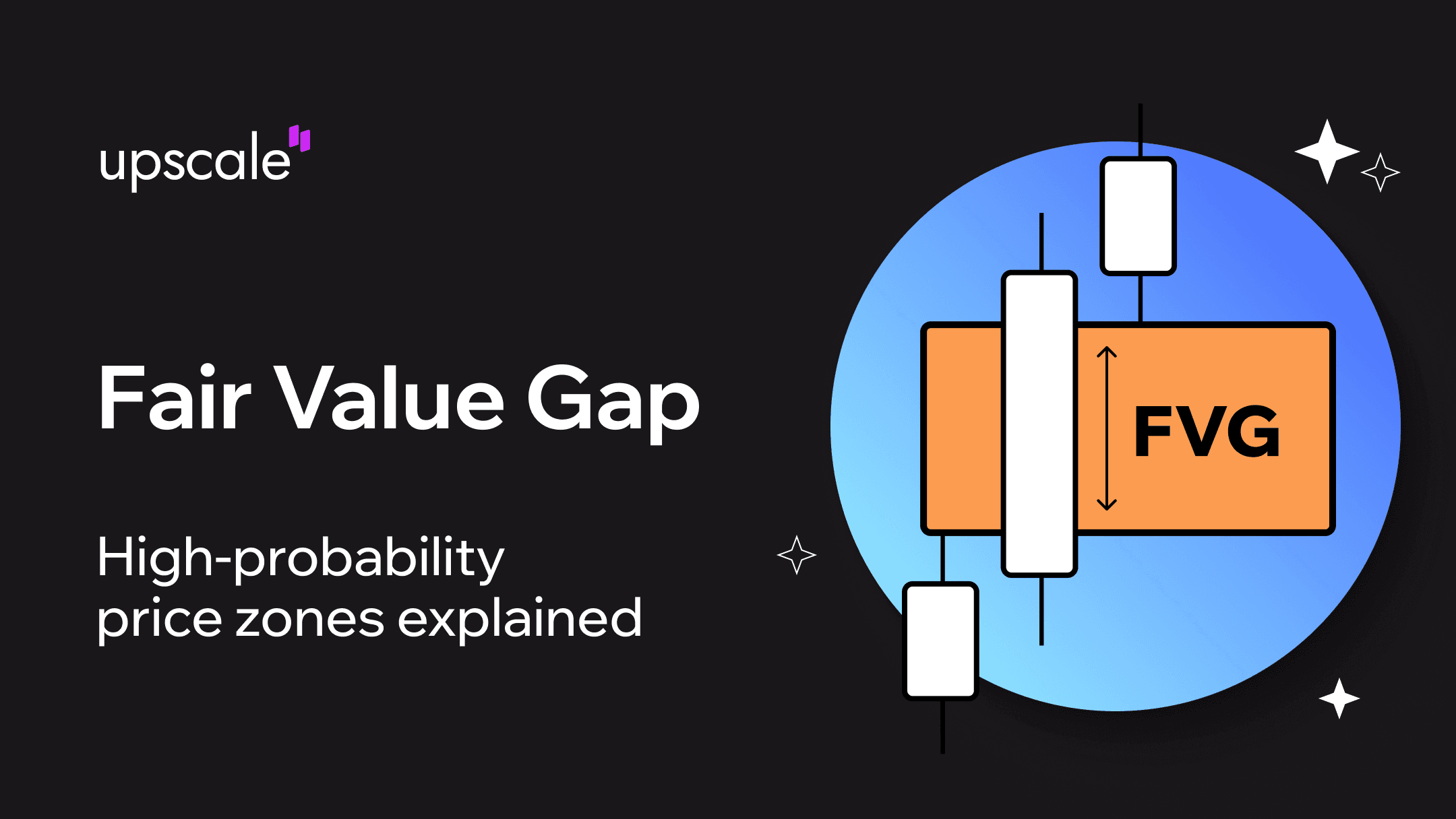
A fair value gap represents an unfilled price zone on your chart. It forms when price moves so fast that normal trading cannot occur. Think of it as a building elevator skipping several floors. Those missed floors wait to be visited later.
Smart Money Concepts framework positions FVGs as powerful tools. They show where institutions entered aggressively. The market remembers these zones. Price returns to them with 70-85% probability.
Why does this matter for you? Because FVGs provide specific entry points. No guessing. No vague support levels. Just clear zones where institutional order flow created imbalance.
When you understand fair value gaps, you stop fighting institutions. You start following them. This guide teaches you exactly how to identify, trade, and profit from these high-probability price zones.
What is a Fair Value Gap in Trading?
Fair value gaps are unfilled price zones on charts. They appear when price moves too rapidly for normal trading activity. The market literally skips certain price levels.
Here is how to spot one. Look for three consecutive candles. The middle candle creates a gap. Its wick does not overlap with the wicks of candles before and after it. This visual pattern appears on any chart.
The formation cause is simple: buyer-seller imbalance. Aggressive institutional orders overwhelm available liquidity. Price jumps to the next liquidity zone. A gap remains behind.
These zones act as magnets. Price frequently returns to fill them. Statistics show 70-85% of FVGs eventually get filled. The market seeks efficiency. Unfilled levels represent inefficiency that must be corrected.
FVGs connect directly to Smart Money Concepts. They represent institutional footprints. When banks or hedge funds move large positions, they leave traces. FVGs are those traces.
Imagine a crowded highway. Everyone suddenly rushes to one exit. Some stretches of road remain empty. Later, traffic flows back to fill those empty sections. FVGs work the same way in markets.
The Market Psychology Behind Fair Value Gaps
Large institutional orders create fair value gaps through aggressive execution. Banks, hedge funds, and algorithmic systems need to move significant positions quickly. They consume all available orders at certain prices.
When institutions buy or sell urgently, they overwhelm liquidity. Price jumps to the next available level. The gap left behind shows where their activity was too aggressive for normal market flow.
Why does price return? Markets seek equilibrium. Unfilled price levels represent inefficiency. Normal price discovery did not occur there. Later participants recognize these zones as institutionally significant.
Technical traders worldwide identify the same FVGs. They place orders near these zones. This creates a self-fulfilling prophecy. More attention means higher probability of price returning.
The result? FVGs act as magnets with 70-85% fill rates. The market rebalances the inefficiency created by institutional urgency.
What Causes Fair Value Gaps in Trading?
Four main catalysts create fair value gaps in trading. Understanding them helps you anticipate new formations.
Institutional order flow is the primary cause. Large players execute significant orders that overwhelm available liquidity. They consume all orders at certain prices. Price skips to the next liquidity zone.
High-impact news events trigger immediate reactions. Fed decisions, employment data, and inflation reports cause rapid price movement. Everyone rushes to the same side. Gaps form as price jumps through levels.
Earnings reports create information asymmetry. Institutions react immediately. Retail traders process information more slowly. This one-sided pressure generates gaps during the delay.
Extreme market sentiment shifts cause herd behavior. Geopolitical events or market crashes evaporate liquidity on one side. Price gaps as it seeks available counterparties.
Note that FVGs relate to supply and demand zones conceptually. However, they differ in precision. FVGs are specific gaps between candles. Supply and demand zones cover broader price areas.
How to Identify Fair Value Gaps on Your Charts
The three consecutive candles rule defines valid FVG identification. Look for three candles where the middle one creates an unfilled gap. The gap should not overlap with surrounding candles.
Follow this step-by-step identification process. First, scan for three consecutive candles moving in the same direction. Second, check if the middle candle created a gap. For bullish FVGs, measure from the high of the first candle to the low of the third. For bearish FVGs, measure from the low of the first candle to the high of the third.
Third, verify that wicks do not overlap. Fourth, measure the gap size. Minimum thresholds vary by instrument. Forex typically requires 10+ pips. Crypto needs 0.2%+ gap size. Fifth, assess market context including higher timeframe direction and recent structure.
Not all gaps deserve your attention. Significant FVGs occur on higher timeframes like 4H and above. They align with higher timeframe trends. They form near key structure levels. They show substantial size relative to average candle range.
Insignificant FVGs appear during choppy price action. They lack directional context. They represent tiny gaps relative to normal volatility. Skip these and focus on quality setups.
Bullish vs. Bearish Fair Value Gap Examples
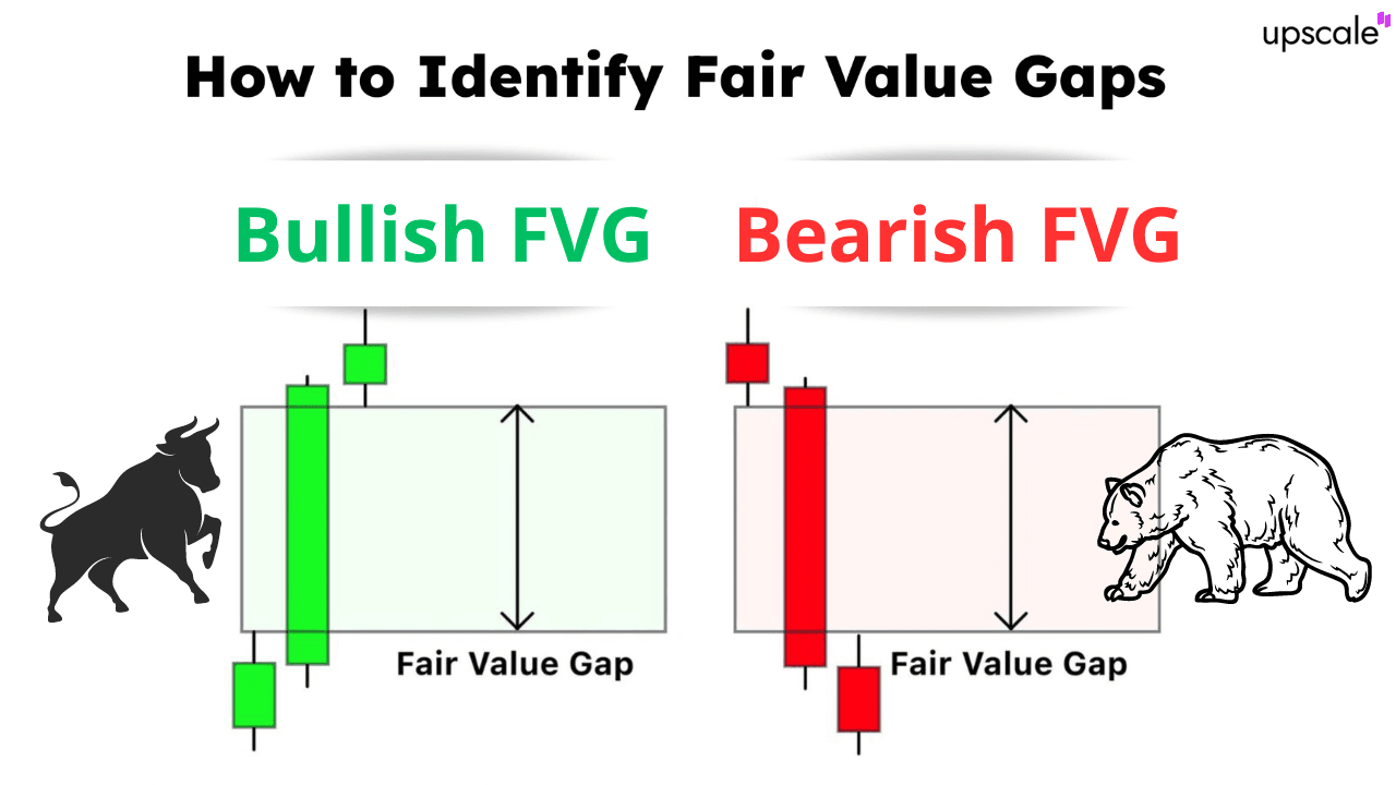 Bullish fair value gaps form during upward price movement. The pattern shows a down candle or consolidation first. An aggressive up candle follows, gapping higher. A continuation candle maintains position above the gap.
The visual result shows unfilled space below current price. This zone represents a long entry opportunity. Price may return here before continuing higher. Target the return to the low of the first candle as minimum expectation. Success rate reaches approximately 75% under proper conditions.
Bearish fair value gaps form during downward movement. An up candle or consolidation comes first. An aggressive down candle follows, gapping lower. A continuation candle does not fill the gap upward.
The visual result shows unfilled space above current price. This zone offers a short entry opportunity. Price may return before continuing lower. Target the high of the first candle. Success rate similarly reaches around 75%.
Both types have comparable reliability. The difference is directional bias. Your selection depends on higher timeframe market structure and your directional bias.
Fair Value Gaps vs. Other Market Inefficiencies
Fair value gaps differ from other market concepts. Understanding distinctions prevents misidentification.
Order blocks represent specific candles where institutions entered. They are the last opposing candle before significant directional moves. FVGs are the unfilled spaces created during the move itself. Order blocks are solid price zones. FVGs are empty price zones.
The relationship matters for trading. Order blocks frequently precede FVGs. Use both together for higher-probability setups. Order blocks show where smart money positioned. FVGs show the inefficiency from their execution.
Regular price gaps differ from FVGs. Regular gaps occur between trading sessions. Think overnight or weekend gaps in stocks. FVGs occur during active trading from rapid intra-session movement. FVGs have higher statistical fill probability at 70-85%.
Supply and demand zones are broader price areas. They span multiple price levels and are less precise. FVGs are specific gaps between consecutive candles. They offer precise, measurable zones. Both reflect imbalances but differ in precision and identification methodology.
Inverse Fair Value Gap Explained
Inverse fair value gaps signal potential reversals. They form at market extremes after extended moves. Price becomes overextended, then reverses immediately.
Standard FVGs suggest continuation or mitigation zones. IFVGs behave differently. They form during the final exhaustion push. Price creates a gap, then immediately reverses through it. This inverts the expected behavior.
Look for IFVGs at obvious extremes. Multi-week highs or lows qualify. Psychological levels and major resistance or support work too. Volume spikes and volatility expansion indicate climactic behavior.
When price immediately rejects its own gap, the previous trend has exhausted. Reversal is underway. IFVG reliability approaches 80-85% due to formation context at significant turning points.
Fair Value Gaps in Different Markets
Fair value gaps manifest across all financial markets. However, market-specific characteristics affect their behavior.
Forex markets show clean FVG formation due to deep liquidity. Major pairs like EUR/USD and GBP/USD work best. Gaps tend to be smaller at 5-20 pips but precise. Best timeframes range from 15-minute to 4-hour charts. Fill rate reaches approximately 75-80% during London and New York sessions.
Cryptocurrency markets display highly visible FVGs due to 24/7 trading and higher volatility. Use 1-hour to daily charts. Lower timeframes can be noisy. Fill rate reaches approximately 70-75%. Larger gaps are common at 0.5-2% for BTC/USDT. Continuous trading means all gaps are true FVGs formed during session.
Stock markets require focus on liquid stocks with high daily volume. Daily to weekly charts generally prove most reliable. Fill rate ranges from 70-80% depending on stock liquidity. Distinguish true intraday FVGs from overnight gaps.
Despite market differences, identification methodology remains identical. Three candles with unfilled gap. Adapt expectations for volatility characteristics of each market.
Fair Value Gap Trading Strategy
A complete FVG trading strategy includes identification, confirmation, entry, stop loss, take profit, and position sizing.
The identification phase locates valid FVGs using the three-candle pattern. Start with 4H or daily charts for clarity. Verify the gap meets minimum size requirements. Confirm it appears in context of higher timeframe trend direction.
Before entry, confirm additional factors. Higher timeframe alignment means FVG direction matches daily or weekly trend. Market structure support shows recent break of structure in FVG direction. Volume context confirms the initial gap formed on above-average volume. Clean price action means no major resistance or support within the FVG zone.
Entry execution offers two approaches. Aggressive entry places a limit order within the FVG zone immediately after formation. This captures best price if gap fills but may not fill if price continues. Conservative entry waits for price to return and show reaction before entering. Confirmation signals include rejection candles, volume increase, or smaller timeframe break of structure.
Stop loss placement goes beyond the FVG zone with a volatility buffer. For bullish FVGs, place stops 5-10 pips below the gap zone. For bearish FVGs, place stops 5-10 pips above. This protects capital if the FVG fails to hold.
Take profit uses a multi-target approach. Target 1 at 50% position goes to the opposite side of the FVG zone. Target 2 at 30% position goes to the next market structure level. Target 3 at 20% position uses extended targets or trailing stops.
Position sizing risks 0.5-1% of account per trade maximum. Calculate position size based on stop distance. Account balance times risk percentage divided by stop loss distance equals maximum position size.
Executing FVG strategies effectively requires proper capital and professional tools. This is where Upscale brings together capital, AI, and precision execution in one prop trading platform.
Professional traders need more than knowledge. They need funded trading accounts with institutional-grade infrastructure. provides exactly that. Transparent terms mean you know what to expect. Risk management infrastructure protects your capital.
The philosophy is simple: we succeed when you succeed. FVG trading in fast-moving crypto markets demands precision execution. Market structure analysis capabilities help identify high-probability setups. With proper backing, you can focus on strategy instead of capital limitations.
Entry and Exit Techniques Using Fair Value Gaps
Entry timing variations affect your results significantly. Choose your approach based on risk tolerance.
Immediate entry places a limit order in the FVG zone right after gap formation. Advantage: captures best price if gap fills. Risk: may not fill if price continues without returning. Best for traders willing to miss some setups for optimal entry when filled.
Confirmation entry waits for price to return and show reaction. Look for strong rejection candles from the zone, volume increases, or smaller timeframe break of structure. Advantage: higher probability as price already shows interest. Risk: may miss quick fills. Best for traders prioritizing higher win rate.
Exit strategies determine your profitability. Fixed targets use the opposite side of the FVG for minimum targets. This represents gap fill with 70-85% probability. Structure-based targets extend to previous swing highs or lows. Scaling takes partial exits at multiple targets. Trailing stops let winners run based on structure.
FVGs serve as price mitigation zones. Price returns to balance inefficiency before potentially continuing its directional move.
Risk Management When Trading Fair Value Gaps
The 70-85% fill rate means 15-30% of setups will fail. Risk management is non-negotiable.
Never risk more than 0.5-1% of total account equity per FVG trade. Calculate position size systematically. Account balance times risk percentage divided by stop loss distance equals maximum position size. Example: $50,000 account with 1% risk equals $500. With a 50-pip stop, maximum position is 10 micro lots.
Always place stops beyond the FVG zone. Never within it. The zone should hold as support or resistance. If it does not, the setup is invalid. Typical stop placement is 5-15 pips beyond gap boundaries depending on volatility. Never move stops further away if price approaches. Accept the loss.
Minimum 1:2 risk-reward ratio is recommended. With 70-85% success rate and 1:2 R:R, mathematical expectancy stays strongly positive. Risk $500 to make $1,000+ creates favorable probability-based edge over time.
FVGs appear frequently. Resist temptation to trade every one. Quality over quantity. Often 2-3 high-quality FVG trades weekly outperform 20-30 lower-quality setups.
Multi-Timeframe Analysis for Fair Value Gaps
Multi-timeframe alignment dramatically improves FVG trading success rates.
 Start with higher timeframes like daily or 4H for direction and major FVGs. Identify overall market trend direction. Find significant FVG zones that institutions likely respect. Note major market structure levels. Only trade FVGs aligned with this direction.
Drop to mid timeframes like 1H or 15M for confirmation and setup refinement. Confirm higher timeframe FVG zones are still unfilled. Identify more precise entry zones within larger FVGs. Look for break of structure toward the FVG. Watch for change of character indicating momentum shift.
Use lowest timeframes like 5M or 1M for entry timing. Execute precise entries when price returns to the FVG zone. Refine stop losses with tighter placement. Spot early exit signals if price action shows rejection.
Break of Structure confirms momentum shift on mid and lower timeframes. Look for BOS in the direction of the FVG before entering. Change of Character on lower timeframes signals that price may return to the FVG zone.
Never trade an FVG on lower timeframes that conflicts with higher timeframe direction. If daily trend is bearish, only trade bearish FVGs on lower timeframes. Ignore bullish FVGs as counter-trend trades. Timeframe alignment often pushes fill rates toward 80-85%.
Real Trading Examples with Fair Value Gaps
Real examples demonstrate how theory becomes practice.
Example 1: Bullish FVG in Trending Market (BTC/USDT)
Market context showed Bitcoin in established uptrend on daily chart with higher highs and higher lows. On the 4H chart, aggressive buying created a bullish FVG between $42,800-$43,200.
Identification showed a clear three-candle pattern. A down candle reached $42,500. An aggressive up candle hit $44,000, creating the gap. A continuation candle maintained position above $43,500.
Entry decision used conservative approach. Waited for price to retrace to the FVG zone. Entry at $43,100 when 1H chart showed rejection candle with volume increase.
Stop placement went below the FVG zone at $42,650 for roughly 1% position risk. First target was $44,500 at recent structure high. Second target was $45,000 at the psychological level.
Outcome: Price reacted immediately from the FVG zone. First target hit within 8 hours. Closed 60% position at $44,500. Moved stop to breakeven. Remaining 40% hit second target. Total weighted gain: 1.4% on full position.
Example 2: Bearish FVG in Reversal Context (EUR/USD)
EUR/USD approached weekly resistance at 1.1000 after extended rally. On the 1H chart, price created a bearish FVG after rejection at resistance.
Aggressive entry placed a limit sell order at 1.0950 expecting price return. Stop placement above FVG zone at 1.0995 for a 45-pip stop. First target at 1.0850 offered approximately 1:2 R:R.
Outcome: Price returned to the gap zone within 6 hours. Filled entry at 1.0950. Then rallied through stop at 1.0995 for full loss. FVG did not hold.
Lesson: The daily chart was still bullish, creating conflict. Counter-trend setups fail more often regardless of FVG quality.
Fair Value Gap Examples Across Different Markets
Market-specific observations help set realistic expectations.
Formation similarity means FVG identification methodology is identical across all markets. Three-candle pattern with gap works everywhere. Size differences matter. Crypto gaps typically run larger at 0.5-2% due to higher volatility. Forex gaps stay smaller at 5-20 pips due to tighter spreads.
Fill rate variations exist. Forex major pairs show 75-80% fill rate due to deep liquidity. Crypto shows 70-75% due to occasional liquidity gaps. Timeframe preferences vary. Crypto works well on 1H-4H timeframes. Forex is optimal on 15M-4H. Stocks work best on daily or higher timeframes.
Execution considerations differ by market. Crypto allows 24/7 trading of FVGs. Forex is limited to session hours. Stocks trade only during market hours.
Common Mistakes to Avoid When Trading Fair Value Gaps
Six main mistakes derail FVG traders.
Trading every fair value gap without context ranks first. Once traders learn FVGs, they see them everywhere. Solution: Implement strict context filters. Only trade FVGs aligned with higher timeframe trend, near significant structure, during high-liquidity sessions, and meeting minimum size requirements.
Ignoring the 15-30% failure rate causes blown accounts. Solution: Accept that roughly 1 in 4-5 setups will lose. Use 0.5-1% risk per trade maximum. Do not abandon strategy after 3-4 consecutive losses.
Entering too early before confirmation stems from impatience. Solution: Wait for price to return and show reaction. Conservative entry produces better results for most traders.
Poor stop loss placement tries to maintain tight stops within FVG zones. Solution: Always place stops beyond the FVG zone with adequate buffer. Accept the loss if the zone does not hold.
Overtrading due to FVG abundance creates temptation to trade continuously. Solution: Set maximum daily or weekly trade limits. Focus on highest-probability setups only.
Trading FVGs in ranging markets ignores market regime. Solution: FVGs work best in trending markets. In choppy conditions, FVG reliability drops. Identify market regime first.
Algorithmic Trading with Fair Value Gaps
Manual scanning across multiple instruments becomes time-intensive. Algorithmic detection offers efficiency.
Automated systems enable simultaneous monitoring of dozens of instruments. They provide consistent identification without human bias. Immediate alerts notify when valid FVGs form. Systematic backtesting validates strategy effectiveness.
Key parameters for algorithmic detection include candle count set to 3 consecutive candles, gap size threshold as percentage of ATR typically at 0.5-1.0x, timeframe settings for 1H, 4H, and Daily, and overlap validation logic.
When backtesting FVG strategies algorithmically, use minimum 2-3 years of data history. Test across trending, ranging, and volatile conditions. Implement realistic execution assumptions including slippage and spread costs. Validate fill rate statistics align with expected 70-85% range.
TradingView offers community scripts for FVG detection. MT4 and MT5 support custom indicators. Algorithmic platforms like cTrader and NinjaTrader enable automated FVG strategies.
Important note: Algorithmic identification does not guarantee profitability. Proper strategy, risk management, and market context understanding remain essential.
Advanced Fair Value Gap Concepts
Fair value gaps do not occur randomly. They represent institutional footprints.
FVGs combined with liquidity pool analysis create high-probability setups. Common pattern: Price sweeps a liquidity pool, taking out obvious stops. Then price aggressively moves away creating an FVG. Eventually price returns to fill the gap. After observing liquidity grab, watch for FVG formation in opposite direction.
Order block plus FVG combinations increase reliability substantially. Order blocks are the last opposing candle before significant moves. When both align at the origin of a move, setup reliability increases. This layered approach often produces 80%+ success rates.
Market structure integration adds significance. Most powerful setups occur when FVG forms immediately after Break of Structure confirming momentum. FVGs appearing near significant swing highs or lows add structural significance. Multiple timeframe FVGs aligning at the same price zone create institutional confluence.
Price delivery algorithms from institutions create predictable patterns. FVGs represent inefficiencies these algorithms later clean up. Understanding this behavior improves anticipation of FVG fills.
Trading Psychology for Fair Value Gaps
Psychological challenges specific to FVG trading require attention.
 Patience is the most difficult psychological aspect. After identifying an FVG, price often continues away for extended periods. Temptation to chase or take poor entries emerges. Solution: Set limit orders and walk away. Missing some trades is better than losing capital on bad entries.
Acceptance of uncertainty matters. The 70-85% fill rate means 15-30% of setups will fail. Each trade feels binary. Solution: View FVG trading as a portfolio of bets. With proper risk management, you can withstand statistical failures while allowing winners to generate overall profitability.
Discipline under pressure tests traders when price approaches the FVG zone. Fear of missing entry, temptation to move entry price, and second-guessing emerge. Solution: Establish entry criteria before price approaches. If criteria are met, take the trade. If not, let it go.
Overcoming confirmation bias prevents seeing FVGs that do not meet criteria. Solution: Use an objective checklist for every potential FVG. If any answer is "no," skip the setup.
Advantages and Limitations of Fair Value Gap Trading
Honest assessment sets realistic expectations.
Advantages of FVG Trading
The 70-85% fill rate provides genuine statistical advantage when properly risk-managed. Visual clarity allows even beginners to identify FVGs with practice.
FVG zones provide natural stop loss placement areas. This creates clear risk definition. Universal applicability means the strategy works across forex, crypto, and stocks on multiple timeframes.
Automation potential allows coding into algorithms for systematic detection. Specific entry and exit points eliminate ambiguity compared to vague concepts. Integration with order blocks, liquidity analysis, and market structure enhances effectiveness.
Limitations of FVG Trading
The 15-30% failure rate is statistical reality. Roughly 1 in 4-5 setups will not work. This requires accepting losses.
Identification subjectivity means valid FVG definitions vary between traders. Minimum size debates continue. Market condition dependency means performance degrades in choppy, range-bound markets.
Patience requirements demand discipline. Temptation to overtrade runs high. Multi-timeframe analysis is necessary for best results. Single-timeframe FVG trading proves less reliable.
Avoid FVG trading during major scheduled news events, extremely low liquidity conditions, clearly ranging markets, and when higher timeframe market structure is unclear.
Conclusion: Implementing Fair Value Gaps in Your Trading
Fair value gaps represent genuine price inefficiencies with 70-85% probability of filling. Proper identification requires the three-candle pattern with unfilled gap between outer candles.
Multi-timeframe alignment dramatically improves success rates. Risk management is non-negotiable since 15-30% of setups will fail. Market context matters because FVGs work best in trending conditions.
Start by practicing identification on historical charts. Then paper trade until your fill rate matches expected 70-85%. Finally, implement with proper position sizing.
The knowledge you now have places you ahead of most retail traders. You understand where institutional money moves. You can identify the footprints they leave behind.
Now practice on a demo account. Mark FVGs on your charts. Track which ones fill. Build confidence through repetition. The edge is real. Your execution makes it profitable.
FAQ
What is a fair value gap in trading?
A fair value gap is an unfilled price zone on charts created when price moves so rapidly that normal trading activity cannot occur at certain price levels. It appears as a gap between three consecutive candlesticks where the middle candle creates space that does not overlap with the wicks of candles before and after it.
How do you identify a fair value gap?
Identify FVGs using the three-candle rule. Look for three consecutive candles moving in the same direction. Check if the middle candle created a gap where its wick does not overlap with the wicks of the first and third candles. Measure the gap size to ensure it meets minimum thresholds for your instrument.
How do you trade fair value gaps?
Trade FVGs by waiting for price to return to the gap zone. Use aggressive entry with limit orders placed immediately after formation. Or use conservative entry by waiting for price reaction at the zone. Place stop losses beyond the FVG zone. Target the opposite side of the gap as minimum profit objective.
What is an inverse fair value gap (IFVG)?
An inverse fair value gap forms at market extremes and signals reversal potential. Unlike standard FVGs that suggest continuation, IFVGs appear after extended moves when price creates a gap during final exhaustion push, then immediately reverses through that gap. They have higher reliability approaching 80-85%.
Do all fair value gaps get filled?
No, approximately 70-85% of fair value gaps eventually get filled. This means 15-30% of FVGs will never fill. Success depends on trading with proper context including higher timeframe alignment, market structure support, and quality setup selection. Risk management accounts for the setups that do not work.
Find more good stuff in our socials
News, tips, and bonuses - come join the crew!
